Introduction
In today's era, we are witnessing progressing volume of attacks and improvement of their sophistication. This can endanger both clients themselves and the shared infrastructure of the data center. For VNET a.s. as a provider of computing and telecommunication services, emphasis is placed on the continuous operation of services, and this leads to motivation for Minerwa project. Our goal is to build a tool suitable, for example, for the SoC team, which will provide an overview of potentially harmful activities in the massive network flow of the data center.
Real-time analysis of anomalies and attacks on a large volume of data flowing through data centers is a complex task. The Minerwa project addresses this issue by employing 2 AI models in layers that analyze network flows. The first layer deals with known attacks and serves as the classification based filter. The second filter instance is represented by an anomaly detector. To improve anomaly detection, we also incorporate diverse characteristics of end nodes in relation to their network communication, specifically clustering them into clusters based on their communication statistics, which enhances anomaly detection performance. In the following sections, we will outline the approach to developing a pipeline for training these AI models and also the solution architecture for the network awareness and early anomaly detection system.
Dataset
The development of AI-based products exhibiting a high level of reliability requires a significant amount of input data. In this section, we want to explain how we obtained and processed data for the purpose of training models capable of detecting malicious traffic.
Data collection and modification
To create an efficient representation of the network traffic and to ensure reasonably fast anomaly detection, we transform the network traffic to network flows. A flow is an aggregated representation of communication between two IP addresses using a particular protocol and ports.
VNET a.s., as an operator of data centers, has access to a large volume of data flowing through border network devices. By mirroring the network traffic from border network devices, we are able to capture specific time intervals and obtain traffic data. As part of the Minerwa project, we have captured two time intervals - approximately 5 days each (August 2022 and December 2022). The captured data was stored in PCAP format, but due to capacity limits, only the first 80 bytes of each packet were saved. The average volume of data in PCAP format amounts to approximately 12 TB per day. PCAP data is exported to the IPFIX format, which is used by the model.
The capture itself does not contain data sufficient for supervised machine learning purposes. Part of the work was focused to inject attack samples into the dataset and label the data. We leveraged an approach involving the artificial generation of attacks in the traffic and injecting attacks into the data itself.
Attack Injecting
A high-quality dataset should contain a great variety of attacks. It is impossible to include each existing attack with all possible parameter settings. Therefore, a suitable representative selection had to be made, so significant part of the project was focused on the research for the dataset posibilities. Representatives of reconnaissance attacks (e.g., scanning), volumetric as well as slow denial of service attacks (e.g., flooding, slow TCP attacks, distributed DoS), exploitation and malware infection communications (e.g., bruteforce, botnet, worm) were included.
For attack injection, multiple methods were used:
- an automated tool for attack injection into the provided captured traffic
- merging of captured attack traffic from another dataset with our own captured background traffic
- synthetic attack generation into the traffic to be captured
Attack Injection Using Injection Tool
Attacks were injected into collected data using the ID2T tool 1, which is a tool for synthetically injecting attacks into existing data in PCAP format. ID2T adjusts the characteristics of the injected attacks based on the characteristics of the existing data traffic (data volume, TTL, MSS, etc.) and does not modify the original traffic. The following attacks were injected:
- Port Scan
- SMB Scan
- MS17 Scan
- SYN Flood DDoS
- SMBLoris
- Eternal Blue Exploit
- Sality Botnet
Attack Injection by Dataset Merging
NDSec-1 dataset 2 covers a set of classic and novel attacks encapsulated within simple but realistic scenarios It includes 14 attack categories. The dataset is available in the form of PCAP captured files and bidirectional flow files in the comma-separated values (CSV) format. We decided to inject following attacks from this dataset:
- Port Scan
- Vulnerability Scan
- HTTP Flooding
- SYN Flooding
- UDP Flooding
- HTTP Bruteforce
- FTP Bruteforce
- SSH Bruteforce
- C&C Command Execution (botnet)
- C&C Communication (botnet)
For the purpose of background cleaning (detection of potential attacks in the captured background traffic, without known synthetically generated attacks), we have injected even more attacks from different existing datasets, namely:
Attack Generation
Besides injecting attacks into the collected data, a set of attacks was generated from our own infrastructure during data capture. We built small infrastructure consisting of several attackers(each attacker identified by distinct IP address) , C&C server and victim to mimic distributed nature of more sophisticated attacks.
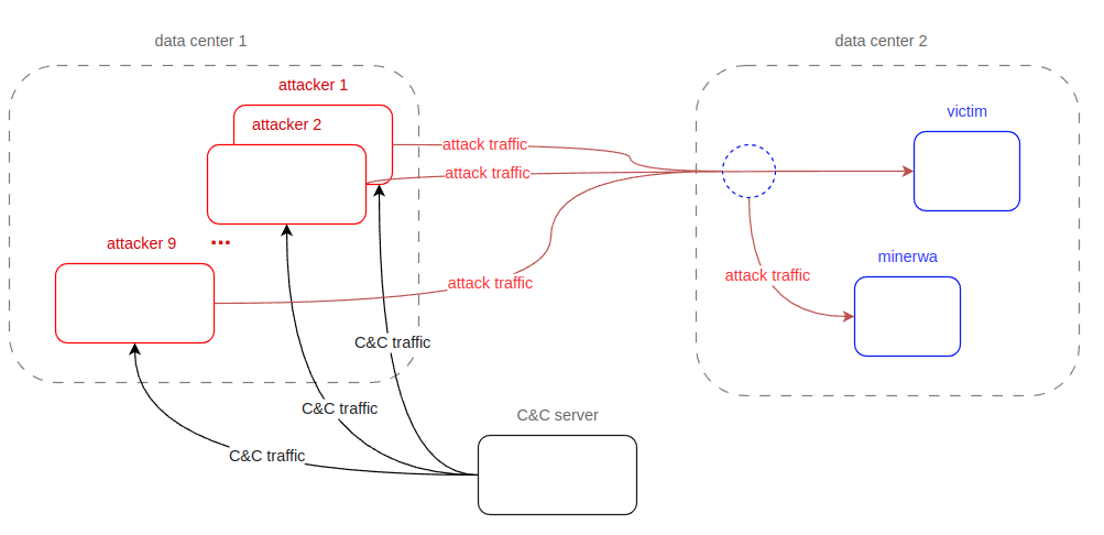
Overview of infrastructure built for attack generation into existing traffic
Picture of infrastructure gives high-level overview of the attack generation. C&C server executes its scenario of attack in distributed manner on attackers. Attackers target one victim which is realized as dummy web server. The main purpose of this infrastructure is to generate pure, easy to label malicious traffic, so there were no other traffic besides traffic from attackers. With precise schedule we are able to label source, destination IP and ports with correct attack label.
The attacks were launched according to a predefined scenario throughout the data collection into the network traffic. Scenario was designed to repeat attacks with variations during different parts of the day. Following types of attacks were generated:
- DDoS Variations (e.g. ICMP Flood, UDP Flood …)
- SYN Flood
- SSH Bruteforce
- HTTP Bruteforce
- URL Enumeration
- Vulnerability Scanning
- Scanning (e.g. XMAS, FIN, UDP …)
Background Filtering
To reach better results with machine learning methods we needed to analyze and detect as many real-world attacks as possible in collected data. For this purpose we leveraged Snort 6 as a tool for known attack detection based on their signatures. When processing captured packets (in PCAPs) we found that Snort produces many false positives. This is probably caused by only capturing the first 80 bytes of each packet. We found the usefulness for traffic cleared by Snort. Even though the false positive rate for attack traffic stayed high, the remaining traffic should better fulfill the definition of benign traffic.
We also trained multiple classification based filters using random forest algorithm (for specific attacks and also general) on already known malign data which were injected or generated.
Using snort and the classificators, we identified 200,084,970 potential anomalies, from which 22,218,676 were known attacks (labeled based on generated attacks in live traffic). In detail:
- Labeled attacks of all flows: 0.2291% (22,250,841 out of 9,712,178,810)
- Predicted attacks of all flows: 2.0601% (200,084,970 out of 9,712,178,810)
- Labeled also predicted: 99.8554% (22,218,676 out of 22,250,841)
The resulting filtered 180M anomalies from the background had to be manually inspected and confirmed by security experts to be labeled as attacks. Due to sheer amount of data we were not able to fully analyze all flows.
Dataset Anonymization
To allow publishing the collected dataset, we need to ensure anonymization of data, particularly IP addresses. We use the method providing prefix-preserving anonymization implemented with nfanon 7 or with yacryptopan 8 in python. The methods use Rijndael (better known as AES), a secure block cipher with 32B (or characters) strong key.
Scenarios
As mentioned earlier, aggregations over packets, so-called flows, were used as the format for input data. Two industry-wide standards for network monitoring protocols, namely Netflow v9 and IPFIX, were considered. For the Minerwa project, we have chosen the IPFIX protocol primarily for its customizability, vendor-agnostic approach supporting the majority of network monitoring tools, and its efficiency and scalability.
The input format dictated the need to find a set of parameters for exporting data from the PCAP format to IPFIX. When choosing parameters, the main focus was on experimenting with data sampling, i.e., determining the ratio of packets used as input for IPFIX exports and aggregations. Other parameters included active timeout and inactive timeout. We experimented with the following set of parameters, where one set was named as the “Scenario”. Parameters for scenarios are present in Table 1.
| Scenario # | Flow direction | Smapling Rate | Active Timeout | Inactive Timeout | Cache Size | Flows Size |
|---|---|---|---|---|---|---|
| 1 | bi-flow | 1 | 60s | 30s | 1M flows | 562 GB |
| 2 | bi-flow | 2 | 60s | 30s | 1M flows | 495 GB |
| 3 | bi-flow | 4 | 60s | 30s | 1M flows | 395 GB |
| 4 | bi-flow | 16 | 60s | 30s | 1M flows | 186 GB |
| 5 | bi-flow | 32 | 60s | 30s | 1M flows | 118 GB |
| 6 | bi-flow | 64 | 60s | 30s | 1M flows | 73 GB |
| 7 | bi-flow | 1 | 30s | 15s | 1M flows | 654 GB |
| 8 | bi-flow | 1 | 2s | 2s | 1M flows | 1.1 TB |
Table 1: Parameters of scenarios and captured size of the collected data per scenario
Purpose of this experiments was to achieve viable compromise between attack visibility and amount of processed data. We performed statistical analysis on the collected data to determine the two most appropriate scenarios to be used for evaluating our anomaly detection detection pipeline.
Statistical Analysis of Scenarios
During the capture, several planned attacks in live traffic were executed. Those attacks were documented and labeled in the captured communication. Additionally, background cleaning was performed on the August capture via trained classification models followed by VNET’s manual expert analysis. Thanks to these steps, the dataset contains more labeled attacks.
During the analysis we discovered that increasing the sampling rate used for scenario generation increases the number of flows with just one packet. Similar shorter timeouts also increase flows with one packet. Both these settings also have significant influence on the deterioration of source and destination IP addresses and hence the flow direction. It is caused by processing other than the first packet of the flow (sampling rate) or cutting longer flows into several flows (timeouts). This was visible mostly in L4 port statistics when there were cases with significantly larger numbers for some ports, even higher as in scenario 1 (a scenario without sampling).
| Sc # | Flows | In Bytes | Out Bytes | In Packets | Out Packets | # of Attack Flows | Size |
|---|---|---|---|---|---|---|---|
| 1 | 13,258,220,557 | 13,258,220,557 | 477,612,141,013,317 | 416,938,581,078 | 484,601,907,115 | 169,892,501 | 562 GB |
| 2 | 11,241,455,572 | 11,241,455,572 | 185,044,097,138,990 | 231,074,408,510 | 209,588,805,059 | 102,342,880 | 495 GB |
| 3 | 9,265,998,957 | 9,265,998,957 | 78,174,026,355,507 | 126,695,677,533 | 96,773,154,190 | 58,623,347 | 395 GB |
| 4 | 4,738,160,378 | 4,738,160,378 | 14,765,296,267,073 | 35,177,305,180 | 20,794,333,261 | 15,794,141 | 186 GB |
| 5 | 3,088,696,018 | 3,088,696,018 | 6,678,072,107,590 | 18,242,179,130 | 9,743,642,307 | 8,018,000 | 118 GB |
| 6 | 1,921,769,207 | 1,921,769,207 | 3,098,308,631,666 | 9,391,346,350 | 4,601,563,595 | 4,046,594 | 73 GB |
| 7 | 16,332,776,598 | 16,332,776,598 | 478,454,474,009,128 | 413,146,176,735 | 482,910,893,549 | 194,634,509 | 654 GB |
| 8 | 31,012,139,384 | 31,012,139,384 | 460,806,118,239,901 | 424,724,103,842 | 472,238,628,838 | 194,924,012 | 1.1 TB |
Table 2: Cumulative flow statistics per scenario from the collected dataset
| Sc # | Flows | In Bytes | Out Bytes | In Packets | Out Packets | # of Attack Flows | Size |
|---|---|---|---|---|---|---|---|
| 1 | 1.000000 | 1.000000 | 1.000000 | 1.000000 | 1.000000 | 1.000000 | 1.000000 |
| 2 | 0.847886 | 0.655065 | 0.387436 | 0.554217 | 0.432497 | 0.602398 | 0.881380 |
| 3 | 0.698887 | 0.384742 | 0.163677 | 0.303871 | 0.199696 | 0.345061 | 0.703147 |
| 4 | 0.357375 | 0.113136 | 0.030915 | 0.084370 | 0.042910 | 0.092965 | 0.330118 |
| 5 | 0.232965 | 0.059044 | 0.013982 | 0.043753 | 0.020106 | 0.047195 | 0.209548 |
| 6 | 0.144949 | 0.030364 | 0.006487 | 0.022525 | 0.009496 | 0.023819 | 0.129528 |
| 7 | 1.231898 | 0.970456 | 1.001764 | 0.990904 | 0.996511 | 1.145633 | 1.165118 |
| 8 | 2.339088 | 1.034443 | 0.964812 | 1.018673 | 0.974488 | 1.147337 | 1.873373 |
Table 3: Cumulative flow statistics per scenario from the collected dataset relative to scenario 1
Table Table 2 and Table 3 shows the visibility of flows. As the sampling rate increases, the number of flows decreases, including attack flows. For example, the sampling rate 1:64 (scenario 6) has only ~2,4% of attack flows compared to scenario 1. Hence, any attack detection method applied on scenario 6, even with 100% success rate, cannot detect more than 2.4% of all attacks that are present in the real traffic. Based on the statistical analysis conducted we proceed to perform evaluation of flow-based anomaly detection for scenario 1 and scenario 3.
Clustering
Background (benign) network traffic is highly diverse. As a consequence, machine learning-based anomaly detection models may have difficulties learning a robust representation of the background traffic, which may result in a higher number of false positives or false negatives. One possible mitigation that is employed and examined in this project is splitting the background traffic into clusters exhibiting similar behavior and training per-cluster anomaly detection models.
There is no single or simple way to divide network nodes into several categories. We recognize two basic categories: home internet users and server housing clients. However, these are not easily distinguishable.
We experimented with grouping VNET nodes (IP addresses administered by VNET) into clusters. Each cluster should contain VNET nodes with similar behavior (e.g., one cluster could contain web servers, another cluster could contain end user nodes). The assumption that anomaly detectors per each cluster exhibit improved performance compared to a single anomaly detector for all VNET nodes.
The description of the network node’s behavior in our case consists of a vector of characteristics describing mainly the volume of data, such as the number of bytes transferred in the port category or the number of unique IP addresses with which the node communicates. The process of node clustering has several steps and is fairly complex. We will provide simplified description of the process:
- Preprocessing - In this step, we aim to eliminate unwanted anomalies, such as flows of injected attacks or remove nodes that have no volume of outgoing communication. Simultaneously, we aggregate data on communication volumes on ports into 13 categories described in the table (see Table 4). The input is IPFIX data, and the output is preprocessed IPFIX flows.
| Port category | Port numbers |
|---|---|
| No TCP/UDP port used | 0 |
| Web traffic | 80, 8080 |
| TLS traffic, probably web | 443 |
| DNS (separate category due to traffic volume) | 53 |
| Email traffic | 25, 26, 109, 110, 143, 209, 218, 220, 465, 587, 993, 995, 2095, 2096 |
| VPNs - L2TP, IPSec, OpenVPN, … | 500, 1194, 1701, 1723, 4500 |
| Data transfer FTP, SFTP, TFTP | 20, 21, 22, 69, 115, 989, 990, 2077, 2078 |
| Shell services - SSH, RSH, … | 22, 23, 513, 514 |
| Playstation Network | 3478, 3479, 3480 |
| IRC chat | 194, 517, 518, 2351, 6667, 6697 |
| Query-response for amplification | 17, 19, 123, 1900, 3283, 4462, 4463, 5683, 6881, 6882, 6883, 6883, 6884, 6885, 6886, 6887, 6888, 6889, 11211, 26000 |
| Dynamic ports | 49152-65535 |
| Other ports | all other port numbers |
Table 4: List of port categories
-
Calculation of node’s statistics per time unit - The input consists of preprocessed IPFIX flows, and the output is the computation of statistics per node per hour. For better description we include some items which are calculated:
- number of source ports per category
- number of destination ports per category
- number of unique (source port, destination port) tuples
- number of unique (destination IP, source port category, destination port category) tuples
- number of incoming bytes (destination to source)
- number of outgoing bytes (source to destination)
- number of incoming + outgoing bytes
- number of flows per VNET node
-
Feature extraction per node - Features are extracted from statistics per hour per VNET IP into a single vector per VNET IP. The output represents extracted features per node. The list below enumerates main features which are extracted:
- Port-based features:
- source port category entropy (from counts of port categories)
- destination port category entropy (from counts of port categories)
- source port category probability (number of input ports per category / # flows per VNET IP)
- destination port category probability (number of output ports per category / # flows per VNET IP)
- Unique tuple-based features:
- Approximate number of unique (source port, destination port) tuples
- Approximate number of unique destination IPs
- Approximate number of unique (destination IP, source port category) tuples
- Approximate number of unique (destination IP, destination port category) tuples
- Approximate number of unique (destination IP, source port category, destination port category) tuples
- Volume-based features:
- incoming and outgoing bytes per hour for work days (24 features in total)
- incoming and outgoing bytes per hour for weekend days (24 features in total)
- incoming bytes / outgoing bytes
- Port-based features:
-
Feature Scaling - All features are scaled before clustering to avoid certain features being dominant. This is important for distance-based clustering algorithms such as k-means where features with high values overshadow features with smaller values. The scaling is realized trough minmax scaling method (0-1 normalization)
-
Clustering - For clustering, we experimented with the k-means clustering algorithm, its hyperparameters, different subsets of extracted features and feature scaling methods. Over 5000 variations of the clustering method were run given all the possible combinations of hyperparameters, out of which we selected a single set of parameters. Based on inertia values for different clustering settings and using the elbow heuristics method on elbow heuristic figure, we selected k-means clustering with 7 clusters.
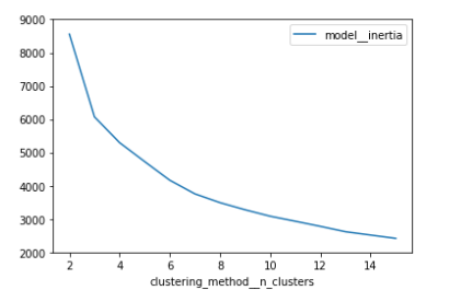
Elbow heuristic figure: Elbow curve based on k-means inertia
We removed IP addresses with a single flow. A single flow does not contain enough information to create a plausible network profile for such IP addresses.
Overview of Used AI Models
We divided the problem of detecting malicious flows in network traffic into the detection of known and unknown attacks. For the detection of known attacks, we used a classification-based model, specifically the random forest. For the detection of unknown attacks (anomalies), we employ a separate anomaly detector.
Classification-based Model
Detection of known attacks is performed by a supervised machine learning model - a classification model, specifically random forest. Supervised learning algorithms require balanced data on input to perform properly. Ideally, each category should have the same amount of incidences. We experimented with three main types of classification, each requiring a different split of data:
- Binary: background and malign flows
- Multiclass: background flows and several specific attack categories (e.g., SYN flood, SSH bruteforce, FIN scan)
- Generic multiclass: background and generic attack categories (DoS, scan, bruteforce, others)
To determine the classification model with the best metrics (accuracy, precision, recall and weighted F1 score) we compared results from all approaches. The best results were achieved for binary classification. We also found out as useful to use binary classification model and forward traffic labeled as malign to be analyzed by second layer multiclass classification model to predict a specific type of attack.
Anomaly Detector
Since the background traffic is highly diverse we awaited that training anomaly detector on entire traffic may not yield satisfactory results, therefore we trained separate anomaly detectors per each cluster. Each detector is trained on network flows pertaining to a cluster of VNET nodes exhibiting similar behavior.
For purposes of anomaly detection we leveraged autoencoder-based models. In this project, we make use of GEE-based variational autoencoders 9.
Architecture of AI Pipeline
As a part of the project we have established architecture for AI pipeline. Both training and prediction pipelines are split into several stages with defined expected inputs and outputs.
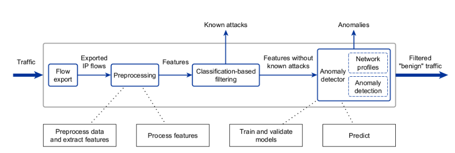
Pipeline architecture figure: Mapping of architecture components to the steps of the anomaly detection pipeline
The pipeline architecture figure illustrates the architecture of the solution. The initial input is the received mirrored network traffic, from which the export to IPFIX protocol flows is generated with a set of parameters described in the scenario section. This export happens ideally on network devices.
The exported IPFIX flows further undergo preprocessing, resulting in feature extraction from the flows per nodes. To improve the efficiency of detection.
A classification-based model is used initially to filter out known types of attacks. Traffic labeled as malicious can then be further processed by a multiclass classification to determine a specific type of attack.
In cases where the classification-based model does not evaluate network traffic as malicious, the extracted features are passed to a module that evaluates anomalies in the traffic. Our assumption was that training separate autoencoders for each cluster of IP addresses would yield better results than the use of a single “universal” autoencoder.
The Network profiles module (in Anomaly detector) requires an input list of VNET’s IP addresses (provided during training phase) and produces a selected number of clusters (profiles) of IP addresses with similar behavior. Based on the Network profiles module, IP addresses are assigned to specific clusters and each cluster has its own Anomaly detection module that is trained on specific cluster features.
The Classification-based filter and Anomaly detector modules can be processed either in parallel or sequentially, depending on the performance requirements. In parallel, the output from the Anomaly detection should be valid only if Classification-based filter does not label a flow as a known attack.
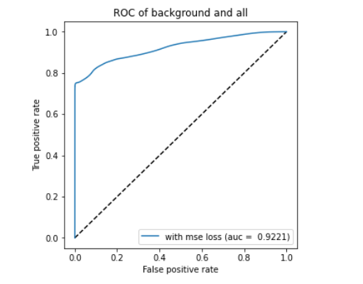
Solution Evaluation
For the evaluation purpose, we have used the AUC ROC metric based on the MSE reconstruction error and KDE plot of MSE reconstruction errors, since these are independent of detection threshold selection. These indications are used for comparison of detection capabilities of detectors for Scenario 1 and Scenario 3 (described in Table 1), as well as for pure anomaly detection(clustered and non clustered form) vs. hybrid anomaly detection.
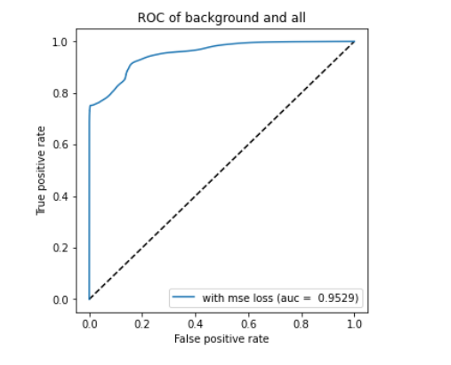
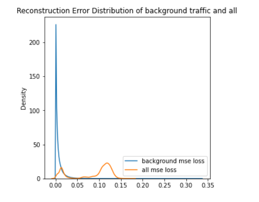
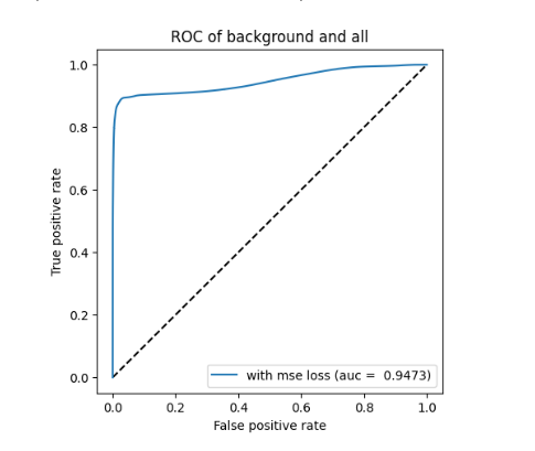
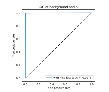
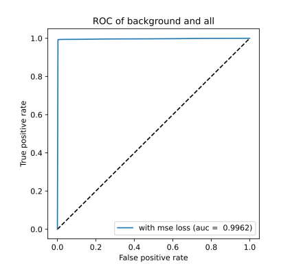
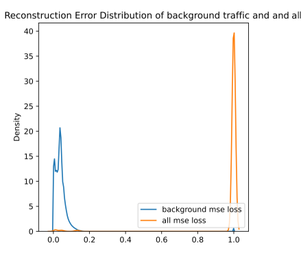
The results are provided in the form of ROC (receiver operating characteristic) and KDE (kernel density estimation) plots based on the MSE reconstruction error. ROC illustrates how the false positive rate increases when the true positive rate increases (higher true positive rate with lower false positive rate is better, i.e., ideally, the curve would reach 1.0 true positive rate while false positive rate remains at 0.0). AUC (area under the ROC curve) is indicating the performance (higher is better, 1.0 is the ideal performance). KDE plot represents estimated distribution of reconstruction errors for background (blue curve) and anomalies (orange curve). The anomaly detection performance is related to how well the curves are visually separable. Overlap means that no reconstruction error threshold is able to differentiate the two (can however trade-off between false positives and false negatives).
Due to the “big data” nature of the crafted dataset (see Section 2) and resource-intensive processes, we are not able yet to evaluate the proposed anomaly detection using all data in time. We chose subset of dataset to do evaluation and training, in more detail we chose three selected hours as a compromise between the time needed for processing and quality of output. . This subset has been pseudo-randomly shuffled and split into train, validation, and test sets, with a ratio of 85:5:10, respectively. To ilustrate volume of data table Table 5 is provided.
| Sample type | scenario 1 train | scenario 1 validation | scenario 1 test | scenario 3 train | scenario 3 validation | scenario 3 test |
|---|---|---|---|---|---|---|
| ALL ATTACKS | 7,300,942 | 419,280 | 842,177 | 3,776,251 | 216,692 | 435,834 |
| ALL SAMPLES | 151,538,503 | 8,710,196 | 17,509,177 | 94,659,600 | 5,441,871 | 10,937,778 |
Table 5: volume of attack labels vs all samples for train, validation and testing for scenario 1 and 3
Train split was used for training of autoencoder-based detectors as well as for training of classification-based filters. Validation split was used for the validation step during autoencoder training as well as for tuning detection thresholds. For the purpose of training classifiers, samples from train split were pseudo-randomly sampled and balanced. Test split was used for evaluation only.
As can be seen from ALL ATTACKS and ALL SAMPLES row of Table 5, the Scenario 3 contains due to packet sampling a lower number of flow records (samples). It contains only about a half of the number of attack-labeled flow records of Scenario 1 and by approximately 40% fewer samples in total, so detection performance in Scenario 3 can hardly outreach performance in Scenario 1 if all communication is taken into account.
Non Clustered Anomaly Detector Performance
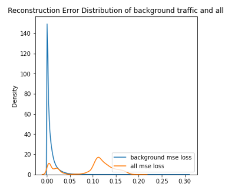
ROC curve based on MSE reconstruction error of non clustered anomaly detector (left/top) and KDE plot of reconstruction errors of non clustered anomaly detector (right/bottom) for Scenario 1
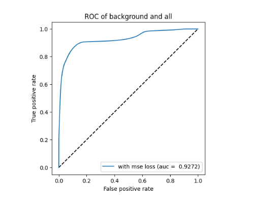
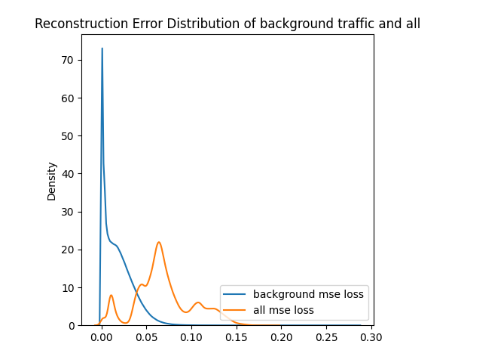
ROC curve based on MSE reconstruction error of non clustered anomaly detector (left/top) and KDE plot of reconstruction errors of non clustered anomaly detector (right/bottom) for Scenario 3
On figures for non clustered ROC and KDE for scenario 1 and non clustered ROC and KDE for scenario 3 we can see that the results are close to each other, while AUC is slightly higher for Scenario 3 (by about 0.005). However KDE plots indicate a more beneficial situation in Scenario 1, where the peak of blue curve is clearer, with lower reconstruction errors (i.e., the autoencoder is better trained).
Clustered Anomaly Detector Performance
ROC curve based on MSE reconstruction error of clustered anomaly detector (left/top) and KDE plot of reconstruction errors of clustered anomaly detector (right/bottom) for Scenario 1
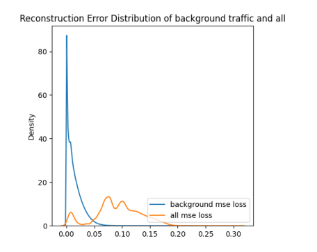
ROC curve based on MSE reconstruction error of clustered anomaly detector (left/top) and KDE plot of reconstruction errors of clustered anomaly detector (right/bottom) for Scenario 3
When compared to single-model anomaly detection in the previous section to the clustered versions on figures for clustered ROC and KDE for scenario 1 and clustered ROC and KDE for scenario 3, we can notice that the AUC is increased by 0.03 for Scenario 1 and by 0.02 for Scenario 3. Thus, the per-cluster anomaly detection can increase the detection performance in general, and our assumption was confirmed.
Results show that even an universal anomaly detection module has significantly better results than expected. Combination of anomaly detection modules for each cluster was still slightly better but in traffic with high volumes we find each improvement useful.
Hybrid Solution Performance
For hybrid detection evaluation, we have combined the trained binary classifiers for both scenarios and combined them with the corresponding trained non clustered anomaly detectors.
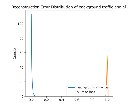
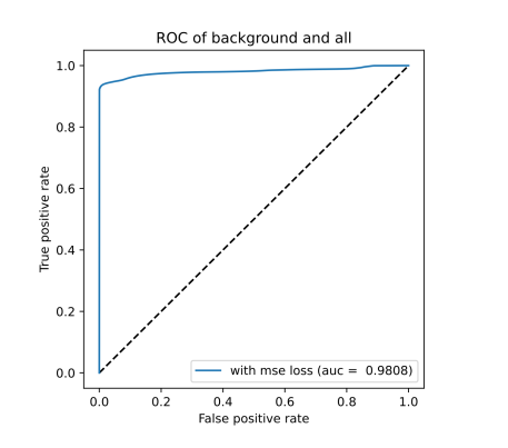
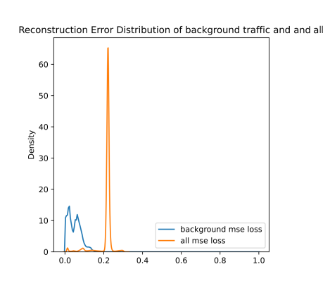
ROC curve based on MSE reconstruction error of hybrid anomaly detector (left/top) and KDE plot of reconstruction errors of hybrid anomaly detector (right/bottom) for Scenario 1
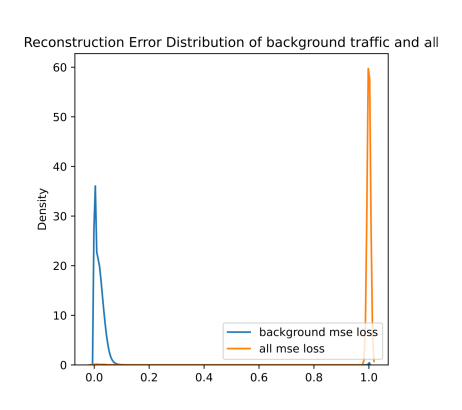
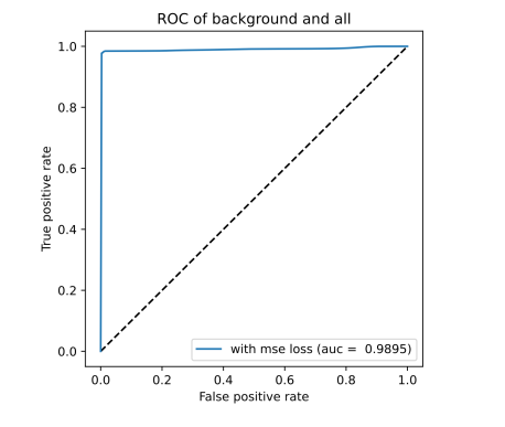
ROC curve based on MSE reconstruction error of hybrid anomaly detector (left/top) and KDE plot of reconstruction errors of hybrid anomaly detector (right/bottom) for Scenario 3
Based on the ROC plots from hybrid ROC and KDE for scenario 1 and hybrid ROC and KDE for scenario 3 figures, it is clear that the usage of the classification-based filter of known attacks is beneficial. The curve is very close to the ideal state for both scenarios. In KDE plots from figures hybrid KDE for scenario 1 and hybrid KDE for scenario 3, we can clearly see that the filter has shifted reconstructions errors of the predicted attacks to 1.0, thus enabling the detector to easily differentiate between the anomalies and benign background. However, we may also notice a shift of some background traffic to 1.0. Thus, the classification-based filter is not perfect and these samples represent either false positives predicted by filter (i.e., background predicted to be an attack) or wrongly labeled background.
For better illustration, following figures shows anomaly-detection confusion matrix for each scenario, which contains absolute numbers. The number in the top-right corner represents false positives and the number in the bottom-left corner represents false negatives.
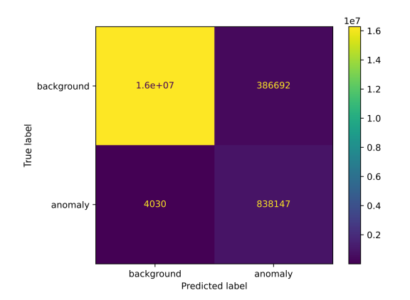
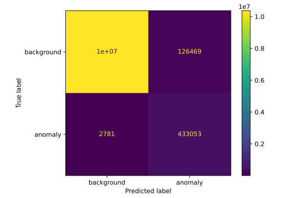
Confusion matrix based on predictions of hybrid detector for Scenario 1 (left/top) and for Scenario 3 (right/bottom)
We proceeded to evaluate performance on data also on December data, more precisely we analyzed 1-hour period in workday at noon time. The goal was to see whether there is a high domain shift in data distribution of the background traffic present between August capture (where training split was taken from) and December capture (where the selected 1-hour was taken from for testing in this experiment). The next goal was to identify whether the trained classification-based filter is able to catch similar “unknown” attacks and if not whether those anomalies are detected by the anomaly detection part.
The results for model trained on august data are worse. Especially, by looking at the KDE plots, we may notice, that the classification-based filter was not able to detect the attacks in Scenario 1 (i.e., the orange curve is not shifted towards 1.0 value). This is not true for Scenario 3, where the filter caught most of the labeled attacks. Based on the blue curve, we may see that the “background” is not located in a single peak on the left (close to 0.0 value). Either the benign behavior is significantly different than in August capture, or there are many unlabeled attacks.
ROC curve based on MSE reconstruction error of hybrid anomaly detector (left/top) and KDE plot of reconstruction errors of hybrid anomaly detector (right/bottom) for Scenario 1 on December dataset
ROC curve based on MSE reconstruction error of hybrid anomaly detector (left/top) and KDE plot of reconstruction errors of hybrid anomaly detector (right/bottom) for Scenario 3 on December dataset
In both scenarios, almost all labeled attacks were detected. Surprisingly, the filter in Scenario 1 did not catch almost any attack, however, it caught almost all in Scenario 3. The reason might be that due to packet sampling, the windowing statistics are less significant in Scenario 3 (i.e., the filter is trained in a more general way).
To conclude this experiment, the domain shift was confirmed, even for a four-months time-frame (between August and December). The domain shift might be also present due to usage of traffic hours for training and December testing (noon hours were not present in the “bigsubset”).
There are several posibilities to decrease negative effects of domain shift. For example retraining the model using the whole August capture will definitely help or if the domain shift is still visible, there is posibility to retrain the autoencoder model each two months.
At the moment we are using already existing pipeline to train more robust model for enhanced detection performance and to lower number of false positives.
Putting it all together
Part of the project is also development of a pipeline for alerting system based on previously described pipeline. We developed pipeline from several components built around previously described AI in order to. The main purpose of this pipeline is to continually feed Minerwa detector with IPFIX flows from collector, store outputs from AI detector, analyze output and execute alerts.
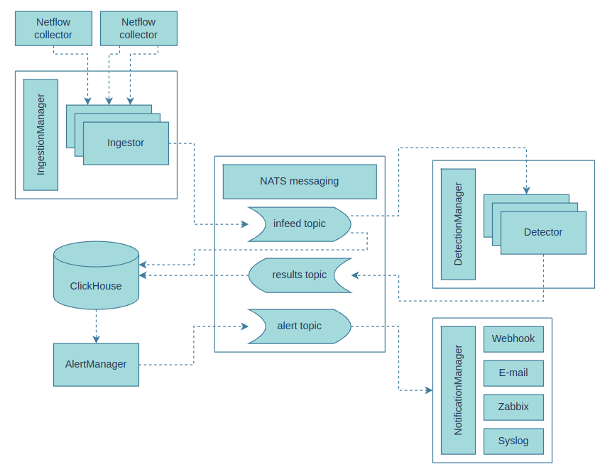
Pipeline architecture for detection and alerting
Figure of pipeline architecture describes the flow in the pipeline. Pipeline flow consists of following steps:
- The input consists of NetFlow/IPFIX data acquired from dedicated NetFlow/IPFIX collectors using ingestors. In this project, we have chosen the nProbe tool for IPFIX data collection, which delivers IPFIX data to our system via ZeroMQ. However, the system can be expanded with additional types of ingestors or implement an ingestor that directly processes network data. It is possible to run multiple ingestors with different configurations, for example, for data collection from various points in the network.
- The output of the ingestors are network flows (NetFlow/IPFIX) represented by an internal data structure, which is further distributed through the NATS system, providing distributed communication based on message queues among different parts of the system.
- Incoming flows from the queue are concurrently written to an analytical database, ClickHouse, and taken for processing by individual detectors.
- Individual detectors, upon a positive finding (such as identifying an attack or anomaly), can send a message with information about the related flow and detected event, which is then recorded in the ClickHouse database.
- Data from the analytical database are continuously evaluated by the AlertManager component, and if an interesting event is identified, a corresponding notification is generated based on defined rules.
- Notifications are processed by individual notification modules according to a selected communication channel. These notifications may not only carry informational value but can also be processed by receiving system as an instructions for action (e.g., blocking network traffic).